Variational Autoencoders with Missing Data
This is a project in collaboration with Jill-Jênn Vie from Inria-Lille, France.
Autoencoders
Dimensionality Reduction
In some applications like data visulization, data storage or when the dimmensionality of our data is to large, we’d like to reduce its dimmensionality of the data, keeping as much information as possible. So we’d like to construct an encoder that takes the original data and transform it into a latent variable of lower dimmensionality. Some times we’d like to recover the original points (with the minimal error) from their encoded versions. So we need an encoder that takes points from the latent space and transform them into points in the original space.
Original/Greedy Autoencoder
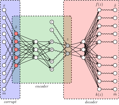
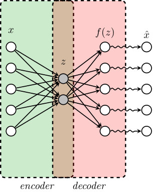
Let’s denote by $x$ an observation in the original space and $z$ its encoded value. If we denote by $g$ the encoder function, then $z = g(x)$. We can decode $z$ through a decoder function $f$, and try to recover the original point from this decoded value. That is, $f(z)$ is not necessarily equal to $\hat x$, this is becasue $f(z)$ does not necessarily belogs to the original space, then we need one more step to transform $f(z)$ into value that belongs to the original space. This final transformation might be done in two different ways, the first and original one is to use a deterministic function that takes decoded value $f(z)$ and transform them into the original space, the second one is to take $f(z)$ as the parameter of a random variable, and make $\hat x$ an observation of this final distribution.
When we model $f$ and $g$ as neural networks (usually deep neural networks), we get the so-called autoencoder. Where $f$ and $g$ are learned with some trainig data set and according to some loss functions $L(x, f(z))$.
Example
For example, if $x$ is an observation of a Bernoulli distribution we could choose $L(x,f(z))$ as the loglikelihood, where $f(z)$ is the parameter of such distribution, that is
$$L(x,f(z)) = f(z)\log(x)+(1-f(z))\log(1-x)$$
where $z = g(x)$ and $f$ and $g$ are learned with (stochastic) gradient ascent.
Note that while $x\in\{0,1\}$, $f(z)\in (0,1)$. Thus, we can take $\hat x = 1\{f(z)>=0.5\}$ (which would be a deterministic approach) or $\hat x\sim \text{Bernoulli}(f(z))$ (which with a random approach), the standard is to take a deterministic approach to go from $f(z)$ to $\hat x$.
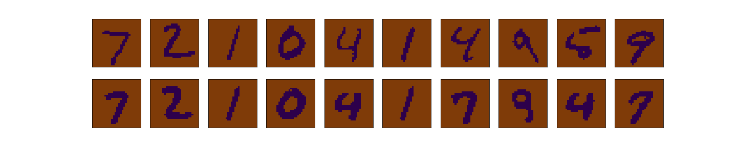
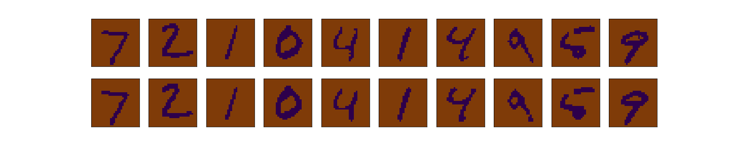
To illustrate this, we consider the MNIST data set, which consist of images of hand-written numbers. The original value of the pixels in each image is between 0 and 1, but we have binarized it, assigning 1 if the value of the pixel is bigger or ueal 0.5 and assigning 0 otherwise. Thus, we can apply the Bernoulli loglikelihood for each pixel. Each image is a 28x28 pixels (thus each image has 784 pixels).The encoder-decoder structure is symmetric, where $g$ and $f$ are multilayer perceptrons, $g$ has two hidden layers of 392 and 192 neurons each layer, and ReLu activation function. The last layer of the decoder has 784 neurons and sigmoid activation function. The latent layer ($z$), has no activation function and we vary the number of nuerons (that is, the dimension of the latent space) in our experiments to be 2 or 98, we denote the dimension of the latent space as $d$.
The next figure shows the structure of our autoencoder. We have preserved this same structure in all our experiments.

< img src=“greedy_ae_latent.gif” title=“Evolution of the Latent Space” width=“300”> < img src=“greedy_ae_latent.png” title=“Final Latent Space” width=“300”>
A good introduction to VAEs can be found here
Irving Gómez-Méndez
Assistant Professor of Artificial Intelligence
I work at the intersection of statistics, machine learning, causal reasoning, and interactive quantitative software.