This page is a state-level exploration of Coneval’s 2018 poverty data for Mexico. The raw data are public and available at Coneval.

The page has three goals:

• give a quick historical context for multidimensional poverty measurement
• explain the subset of indicators used here
• build an interpretable poverty ordering of Mexican states

History

Human Poverty Index

Before the Multidimensional Poverty Index, poverty was often summarized through the Human Poverty Index (HPI), introduced in 1997 as a complement to the Human Development Index.

There were two versions:

• HPI-1 for developing countries
• HPI-2 for high-income OECD countries

A short reference is available at https://en.wikipedia.org/wiki/Human_Poverty_Index.

Multidimensional Poverty Index

In 2010, poverty measurement moved toward a multidimensional framework. Mexico played a central role in that transition through Coneval, the autonomous institution responsible for evaluating social development policy.

History of the Multidimensional Poverty Index in Mexico

The full story is documented by Coneval at this report. The short version is:

1. In 2001, the Mexican federal government organized the symposium Pobreza: Conceptos y Metodologias because there was still no consensus on how poverty should be measured.
2. The same year, the CTMP was created to design an official indicator.
3. That indicator was expected to be:

• simple to communicate
• consistent with common sense
• statistically robust
• easy to replicate

1. Early official indicators appeared in 2002 and 2004.
2. Distrust in government statistics helped motivate the creation of Coneval, which began operating in 2006.
3. From 2006 onward, Coneval built the conceptual and statistical framework for multidimensional poverty measurement using INEGI data sources such as the MCS and ENIGH surveys.

The key methodological shift was clear:

• poverty should not be reduced to income alone
• social rights and economic well-being should be analyzed together
• the framework should remain transparent and reproducible

Coneval’s formal methodology is documented here:

Methodology for the multidimensional measurement in Mexico

Mexico was the first country to implement this approach nationally, and related versions later influenced poverty measurement in several other countries as well as the UN framework adopted in 2010.

Data Analysis

About the Data

This is my own analysis of the 2018 Coneval data. It is inspired by the official framework, but it is not the official Coneval methodology for computing the multidimensional poverty index.

For this page I work at the state level and focus on 10 indicators. I group them into two main blocks.

Social Rights

• Basic education (ic rezedu)
• Access to health services (ic asalud)
• Access to social security (ic segsoc)
• Home’s quality and space (ic cv)
• Access to basic services at home (ic sbv)
• Access to quality food (ic ali)

Two derived indicators summarize whether these deprivations accumulate:

• Privation (carencias). This equals one when a person lacks at least one of the previous social rights.
• Extreme privation (carencias3). This equals one when a person lacks at least three of the previous social rights.

Economic Well-being

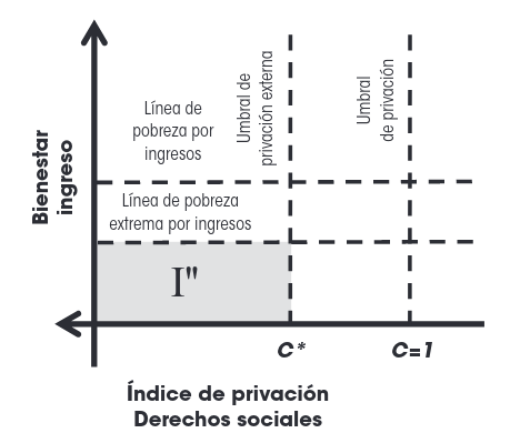
Income is translated into two poverty thresholds:

• Poverty line by income (plb). This equals one when income is insufficient to cover basic needs.
• Extreme poverty line by income (plb m). This equals one when income is insufficient even for basic food needs.

Coneval also tracks broader inequality variables that I do not use on this page, for example:

Society

• Gini coefficient in income
• Access to paved roads

The combination of income poverty and social deprivation creates four broad situations:

• Category I: income above the poverty line and no deprivation.
• Category II: income above the poverty line, but with some deprivation.
• Category III: no deprivation, but income below the poverty line.
• Category IV: income below the poverty line and with deprivation.

If we replace the basic thresholds with the extreme ones, we can isolate extreme poverty.

My Analysis

The autoencoder (AE) and the construction of a poverty index

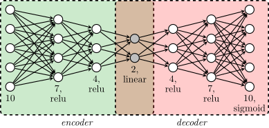
The starting point is simple: each state is represented by a 10-dimensional vector containing the average value of each indicator.

To anchor the space, I added two hypothetical entities:

• Dystopia: nobody has access to the relevant social rights and everyone falls below the extreme poverty line
• Utopia: everyone enjoys the social rights and nobody falls below the poverty line

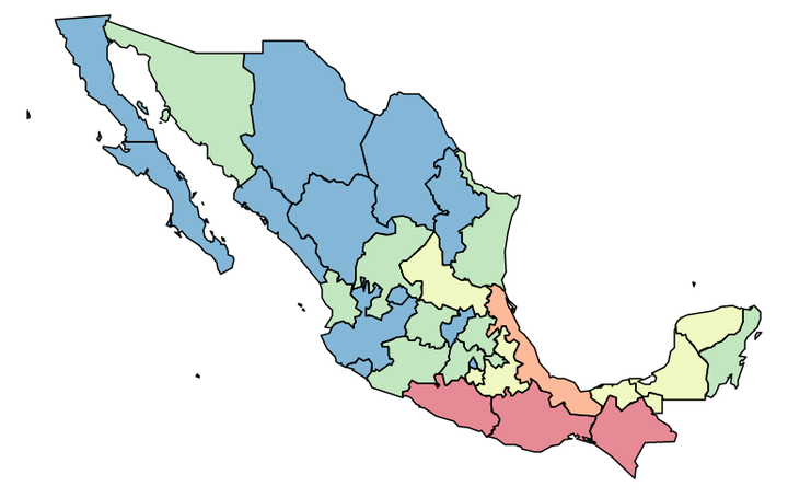
I then trained an autoencoder on the states plus those two reference points. The purpose was not prediction, but representation. The encoder learns a compact two-dimensional space where the states line up in a way that follows common sense: the more industrialized northern states lie closer to Utopia, while poorer southern states lie closer to Dystopia.

From that latent space, I took the first principal component and used it as a one-dimensional poverty scale. I call the result the AE poverty index:

• Utopia is normalized to 0
• Dystopia is normalized to 1
• each state receives a value based on its position along that line

The next plots show that latent-space ordering and the induced index.

AE poverty index

Use of PCA to explain the poverty index

The weakness of the autoencoder approach is interpretability. It gives a sensible ordering, but not a simple explanation of why that ordering appears.

To make the result more interpretable, I also ran a PCA on the same 10-dimensional state vectors and kept the first two principal components. This gives a linear approximation of the data and allows a biplot.

The main takeaways are:

• the first principal component behaves like a weighted average of deprivation variables
• Access to basic services at home has the strongest loading, suggesting that it captures one of the largest dimensions of inequality across states
• Access to health services has the weakest loading, suggesting less variation across states for that indicator
• the second principal component is harder to interpret, especially because both Dystopia and Utopia fall on the same side of it

So I treat the first component as informative and the second one with caution.

PCA, colors considering Dystopia and Utopia

Histograms

These histograms focus on five variables that I consider especially important to reduce: privation, extreme privation, poverty by income, extreme poverty by income, and lack of food.

Boxplot

The boxplot summarizes the same indicators in a more compact way. It makes medians, spread, and outliers easier to compare at a glance.